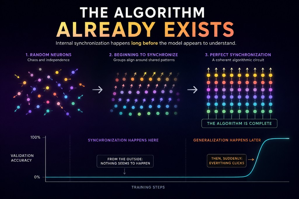
TL;DR: Grokking looks sudden from the outside. Internally, the algorithm can finish organizing long before validation accuracy rises. That gap is mostly regularization, not more computation — and once you can detect the early sync point, you can intervene.
One of the strangest discoveries in deep learning is grokking.
A neural network memorizes training data for thousands of optimization steps.
Validation accuracy stays near random.
Then, almost instantly, it jumps to nearly 100%.
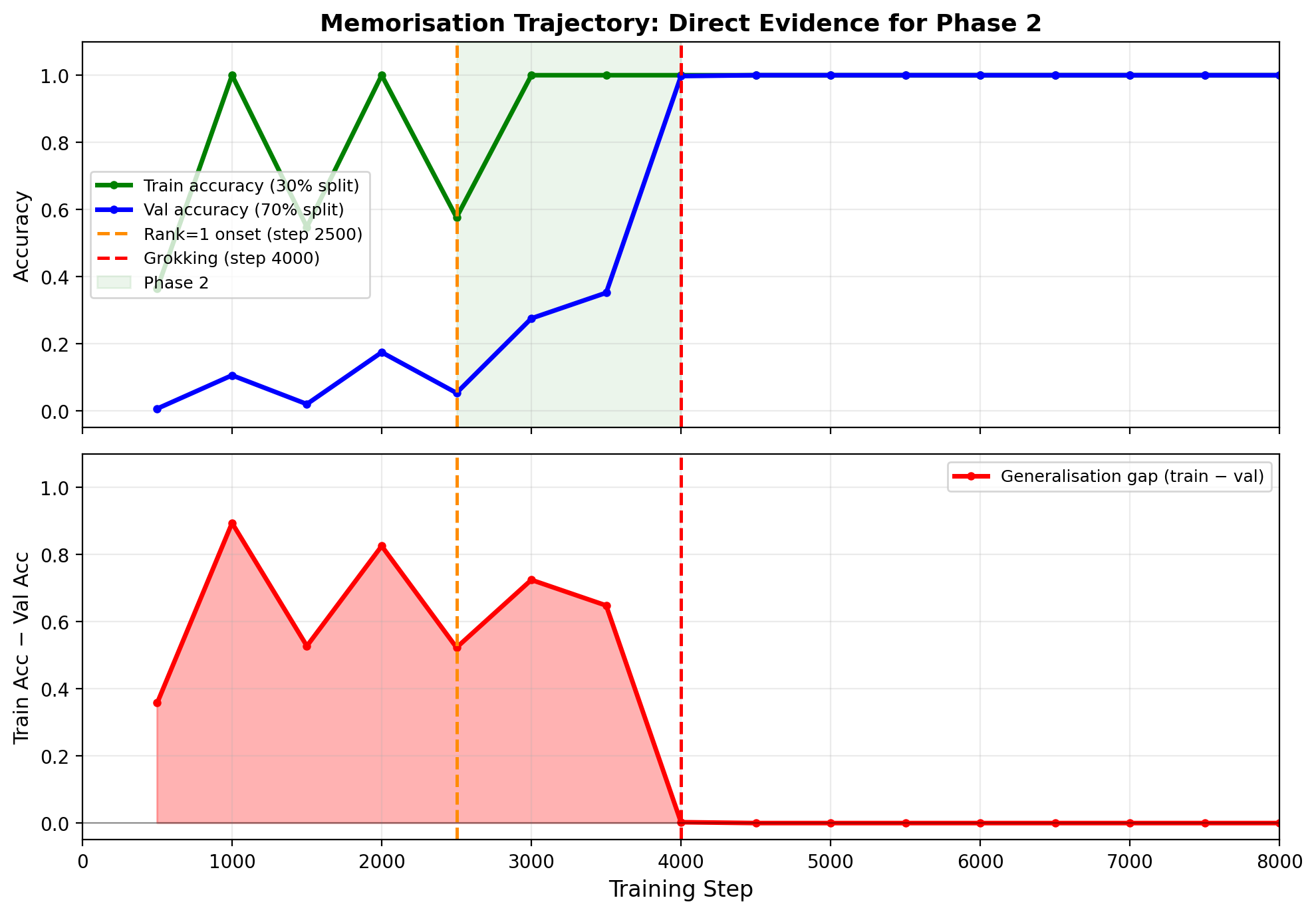
The network somehow discovers the correct algorithm — but only long after it already seemed to know enough to solve the task.
For years, we understood what the final algorithm looked like.
But one question remained unanswered:
When does that algorithm actually appear?
This post is the story of how we chased that question — including the part where the first results looked wrong.
Paper: Circuit Synchronization Precedes Generalization: A Causal Precursor to Grokking.
Everyone looked at grokking backwards
In 2022, Power et al. showed that transformers trained on modular arithmetic can memorize for a long time and then suddenly generalize. The phenomenon was dramatic enough to get a name: grokking.
Then Nanda et al. (2023) opened the black box. For modular addition, they showed what the final solution looks like: a compact algorithmic circuit that exploits sinusoidal structure.
That work answered a crucial question:
What does the finished algorithm look like?
What it left open was different — and harder:
When does that algorithm appear?
Most progress measures watch the output of learning: accuracy, loss, or restricted losses that already assume we know what to look for.
We wanted something closer to the internal event itself:
the moment neurons stop behaving like independent memorization machinery and start behaving like a shared algorithm.
An orchestra before the performance
Imagine watching an orchestra warm up.
At first, every musician plays independently. Notes collide. There is no piece yet — only noise.
Gradually, more players lock onto the same rhythm.
Eventually the music emerges.
Existing work on grokking mostly notices the final performance: validation accuracy leaping upward.
We wanted to know something quieter:
Can we detect the orchestra synchronizing before the audience hears anything?

That intuition became Frequency Synchronization Degree (FSD).
A simpler picture of FSD
Before the formal definition, here is the picture that helped us most.
Imagine 512 people in a stadium.
Everyone holds a colored card.
Early in training, the cards are random — every color everywhere.
Halfway through, little groups form. Islands of the same color appear.
Eventually, almost everyone is holding the same color.
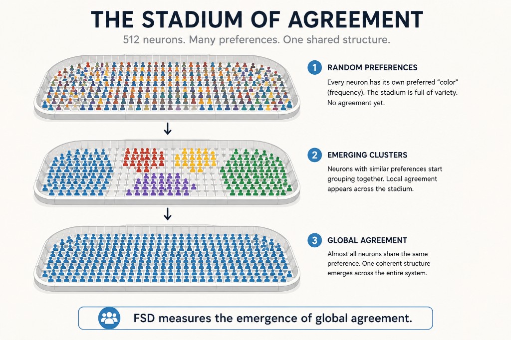
That alignment is what FSD tries to measure.
More precisely, for modular arithmetic, each neuron develops a preferred frequency — a preferred “color.” FSD tracks how strongly those preferences synchronize into a shared computational structure, relative to chance. It does not require a hand-picked list of key frequencies up front.
The point is not the formula.
The point is the chronology:
synchronization can finish while the model still looks, from the outside, like it understands nothing.
The first plots looked like a bug
We expected FSD to roughly follow validation accuracy.
Rise together.
Peak together.
That is not what happened.
In the first run, FSD climbed early — and then sat near its maximum while validation accuracy stayed near chance for a long time.
It looked wrong.
So we checked the logging.
Then the checkpointing.
Then the metric implementation.
Then we trained another model.
Then another.
Eventually we realized the code was not wrong.
The models were telling us something we did not expect:
the internal organization was finishing first.
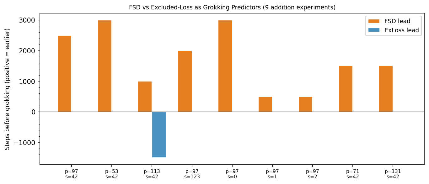
Across nine modular-addition configurations (five primes, three seeds), synchronization reached its post-grokking level 500–3,000 steps before validation accuracy jumped. The mean lead was 1,722 training steps. Every configuration was positive.
It was also earlier than a restricted-logit / excluded-loss style baseline in all nine cases.
Once you trust that curve, the mystery changes shape.
The network is not suddenly becoming capable at the accuracy jump.
Something algorithmic is already there.
So the better question becomes:
The model already knows the algorithm
This is the claim that still feels shocking when I say it out loud.
By the time FSD hits its ceiling, the model already knows the algorithm.
It has already discovered a solution.
It simply has not stopped relying on memorization.
That is why the outside still looks stuck.
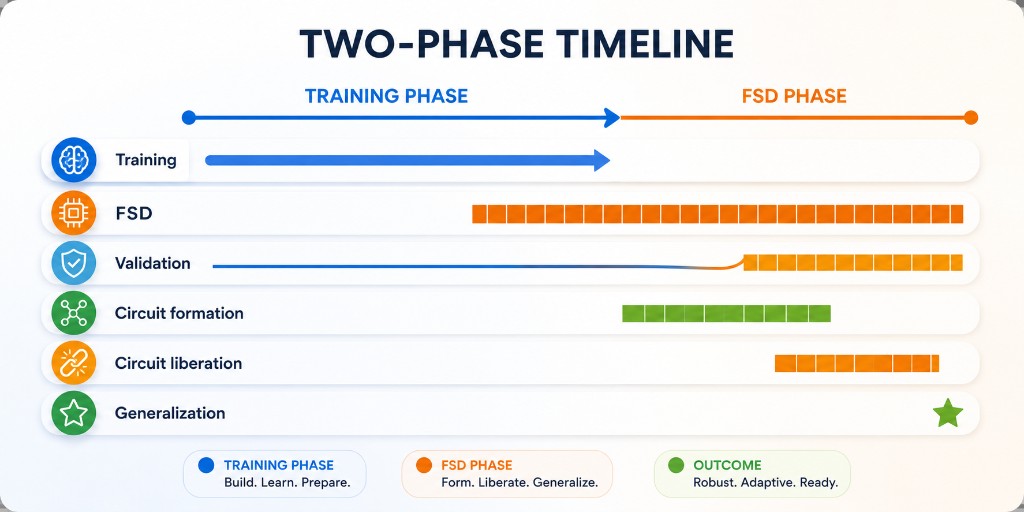
Grokking is not one phase.
It is two.
Phase 1 — Circuit formation
Neurons align. Representations compress. The shared algorithm becomes computation-complete.
From the outside: low training loss, poor validation accuracy.
From the inside: the orchestra has already found the score.
Phase 2 — Circuit liberation
Memorization is cleaned away under regularization. The memorization gap collapses. The already-formed algorithm is finally free to dominate behavior.
Only then does validation accuracy leap.
In one sentence:
Phase 1  →  the algorithm appears
Phase 2  →  memorization disappears
Then     →  generalization becomes visible
This picture is supported by the usual companions of cleanup: rank collapse during formation, weight-norm changes during liberation, and the collapse of the memorization gap at grokking.
But correlation is still not enough.
If Phase 2 is really regularization — not more circuit building — we should be able to intervene.
A risky prediction
If we were right, then we should be able to pause training exactly when FSD peaks.
At that moment, the algorithm should already exist.
So changing only the regularization should shift the grokking time — without needing to rebuild the circuit itself.
That prediction is unusually risky.
It could have failed immediately.
It did not.
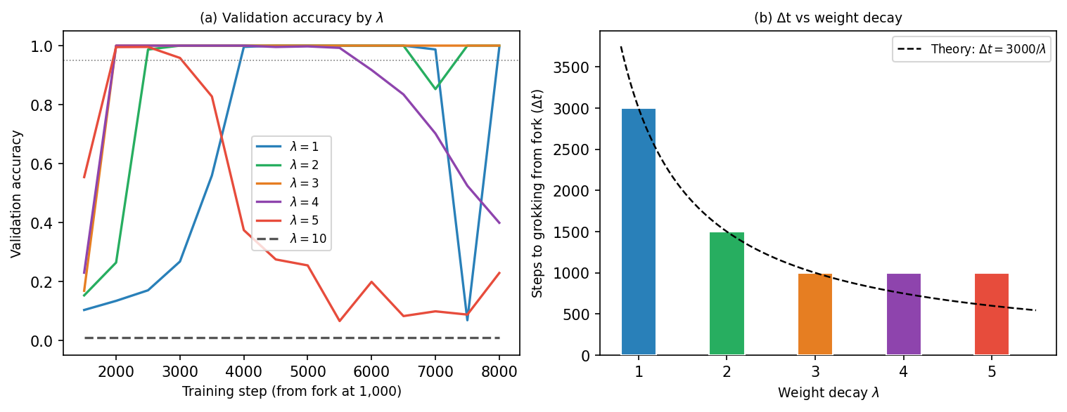
We forked training at the FSD-ceiling checkpoint.
Same weights.
Same synchronized internal structure.
Different weight decay.
Then we watched.
For stable branches, higher weight decay produced monotonically earlier grokking, with remaining time-to-grokking approximately inverse in weight decay:
Higher λ  →  earlier grokking
Δt ≈ C / λ
In plain language:
the algorithm itself was already complete thousands of optimization steps before the model appeared to generalize.
Only the rate of memorization decay determined when that hidden competence became visible.
For modular addition, that completed algorithm is a Fourier circuit. But the important claim is broader than the name of the circuit: computation finished early; cleanup finished late.
That is what turns a progress measure into a causal story.
“Isn’t this just Fourier cheating?”
Fair question.
If you invent a Fourier-flavored detector and then apply it to a Fourier solution, maybe you are measuring your own assumption.
So we changed the task.
On the non-abelian group S₅, the solution does not live in simple 1-D Fourier modes. It lives in multi-dimensional irreducible representations.
There, the original Fourier reading of FSD fails as a precursor.
But a basis-faithful generalization — read in the task’s actual representation basis — still precedes grokking across seeds.
That is the result that made the phenomenon feel fundamental:
Not “Fourier detector finds Fourier thing.”
Instead: “Task-faithful synchronization precedes generalization.”
Why this might matter
The useful framing is not “we invented a metric.”
It is:
Imagine training systems that continuously monitor internal organization.
Instead of blindly waiting for validation metrics to move, they could notice when useful computation has already emerged — then change optimization accordingly.
Our experiments already sketch one concrete version of that idea.
When FSD reaches its ceiling, increasing weight decay can accelerate grokking substantially — about 36–43% faster than a fixed schedule in our setting — without the instability we saw from poorly timed memorization triggers.
That is a small prototype of a larger hope:
Train less blindly. Notice when the algorithm is already there.
Closing
Grokking has always looked like a sudden breakthrough.
Our experiments suggest something quieter.
Neural networks don’t suddenly become intelligent.
They slowly organize themselves into an algorithm while appearing to make no progress at all.
By the time validation accuracy jumps, the important work is already over.
We simply hadn’t been looking in the right place.